Consider the operations of a hypothetical company – Total Toy. Total Toy is a retailer that can sell a total of 14,400 dolls for $30 each.[1] It buys dolls from its supplier for $24 each.[2] It is a magical enterprise that can do this without paying any landlords or workers – Cost of Goods Sold is the only expense.
How would this “value generating engine” would be portrayed in an economics class? There, the focus would be on whether Total Toy creates value, and if so, how it can maximize the value created. The basic idea would be to define revenue and cost as functions of “volume” and see whether profits are positive for any volume and at what volume they are maximized.
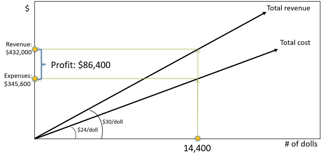
Executing this strategy is extremely simple for Total Toy. Total revenues would be equal to $30 times the number of dolls sold. Total costs would be $24 times the number of dolls sold. Here’s a picture:

It is worth going into great detail about the construction of this graph. The idea of the graph is to depict the value-generating possibilities of Total Toy.
The y-axis is labeled $, but what exactly is meant? Economists would want the y-axis to reflect the dollar amount of the value produced. Whether this value is manifested in cash, or the right to collect cash (i.e., receivables), is of no concern to an economist. (It will be to us!)
The x-axis is labeled # of dolls. What exactly do we mean by this? In the case of Total Toy, there are three possibilities: the number of dolls purchased, the number sold or the number held in inventory. Of these three possibilities, the number of dolls sold is the most directly related to the process of value creation. Once we designate a time period, we choose the point along the x-axis corresponding to the number of dolls sold that period. We then look vertically up from there to the total revenue function, which gives us the value received by Total Toy for the number of dolls sold that period. In accounting language, we have just applied the process of revenue recognition.
Continuing to use accounting terminology, to complete the assessment of profit, we now need to match expenses to the revenue recognized. In terms of the graph, proper matching consists of choosing the point on the x-axis corresponding to the number of dolls sold, looking vertically up to the total cost function and then reading the costs off the y-axis.

The final step is to calculate the dollar amount of the net value generated. In the figure below, $ Profit is the dollar value of the net value created in the period and is the difference between the dollar amount of revenue recognized and the dollar value of costs matched against that revenue.
These figures provide a compelling picture of Total Toy’s opportunities to generate value in a period. Note that there is an implicit distinction between Total Toy and other entities in the society. Sales must be to entities other than Total Toy (i.e., a customer), and the revenue recognized by a sale is the dollar amount agreed to by both Total Toy and each of its customers. Similarly, expenses match against these revenues are linked to the dollar value of transactions in which Total Toy was the customer and other entities were suppliers. Therefore, these figures provide a model of the interactions of Total Toy with two other sets of actors: customers and suppliers. Like any model, a great many details are suppressed. In particular, the mechanics of the transactions between Total Toy, its customers and its suppliers are left out. We will fill in some of these details later, but first, it is worth considering one more “big” question.
Value of Total Toy
Now let’s think about the value of the enterprise, Total Toy. The value of Total Toy is a rather abstract thing. It is the value of the opportunity to generate value by operating Total Toy over time. To assess that, we turn to the techniques of modern finance.
The first thing we should notice when we find the relevant chapters in our finance test is that the value of Total Toy is viewed as being determined by the properties of the stream of cash flows it generates for its owners. Three properties of this cash flow stream are important: their amounts, their timing, and their riskiness. For our current purposes, we can suppress issues of risk and focus on amounts and timing. In particular, let’s adopt the straightforward view that the value of Total Toy is the present value of the cash flows it could generate to its owners.
It is important to observe that the figures presented so far do not directly address Total Toy’s cash flows. They address value flows. To get at cash flows, we must fill in some details as to how Total Toy operates; i.e., how more precisely Total Toy’s value generation opportunities are exploited. A natural place to start is to flesh out the transactions between Total Toy, its customers and its suppliers.
[1] In terms of a traditional demand curve, our assumptions are pretty extreme. In any period, 0 dolls are demanded at any price over $30. Further, cutting the price to, say, $29, is assumed to result in no additional demand.
[2] The implicit assumptions about the supply curve are also extreme. At any price below $24, zero dolls will be supplied, and any number of dolls will be supplied at $24.